This blog post is related to my Google Summer of Code 2024 project: Procedural Fragment Shader Generation Using Classic Machine Learning.
After installing Arch Linux, I plan to build RGM as a productive task during this period. Naturally, it won’t run successfully on the first attempt, so I’ll document the error here for future reference:
    [ 76%] Linking CXX executable emake
    /usr/bin/ld: CMakeFiles/emake.dir/EnigmaPlugin.cpp.o: undefined reference to symbol '_ZN4absl12lts_2024011612log_internal21CheckOpMessageBuilderC1EPKc'
    /usr/bin/ld: /usr/lib/libabsl_log_internal_check_op.so.2401.0.0: error adding symbols: DSO missing from command line
    collect2: error: ld returned 1 exit status
    make[2]: *** [Submodules/enigma-dev/CommandLine/emake/CMakeFiles/emake.dir/build.make:203: Submodules/enigma-dev/CommandLine/emake/emake] Error 1
    make[1]: *** [CMakeFiles/Makefile2:625: Submodules/enigma-dev/CommandLine/emake/CMakeFiles/emake.dir/all] Error 2
    make: *** [Makefile:136: all] Error 2
Before installing Arch Linux, I attempted to build RGM on my Ubuntu machine, but encountered the same error. This was before I was accepted into GSoC.
During the bonding period, I wasn’t able to contribute much, as I was occupied with my final exams.
Later in the bonding period, specifically on May 24th, I wanted to begin writing some code but was unsure where to place it, as the overall project structure was still unclear.
In any case, the graph backend isn’t directly related to the Graphics_Systems, although it will require a system for rendering the generated shaders. After some thought, I concluded that the most suitable location for it would be within the Universal_System, and Josh agreed with this placement.
Here’s the expected structure of my files:
enigma-dev
├── ...
├── CommandLine
│   ├── ...
│   └── emake-tests
│       ├── ...
│       └── ShaderGraphTests
│           ├── ...
│           ├── GraphTests.cpp
│           └── NodeTests.cpp
└── ENIGMAsystem
    └── SHELL
        ├── ...
        └── Universal_System
            ├── ...
            └── ShaderGraph
                ├── ...
                ├── Graph.cpp
                ├── Graph.h
                ├── Node.cpp
                └── Node.h
Once the graph is implemented, I will move on to developing the generator. However, I’m unsure how I will visualize the output shader. I’ll discuss this with my mentor, but there’s a possibility that I might need to integrate the node editor with RGM, which I would prefer to avoid.
Machine Learning Role
Machine Learning can seed the texture octaves based on keywords like grass or clouds. Check: https://filterforge.com/. NeoTextureEdit is another example of a tool that uses machine learning to generate textures, however it is Java. Those doesn’t use machine learning to generate the shaders, but they can be used as a reference. These are toolboxes for converting noise into textures. For example:
-
They can assign functions to bands of values from the noise (e.g. 0 - 0.5 are this color/texture/function, values above 0.5 are this other one)
-
They can use your noise as, e.g, bump maps, height maps, normal maps, spec maps, etc.
Also, an LLM can be used on top of this to choose noise kernels and parameters. See https://upload.wikimedia.org/wikipedia/commons/c/ca/Examples_Of_Filter_Forge_Textures.png.
This is related to RGM and ENIGMA as well, because we want the compositor functions to be available in the engine so users can ship those instead of the image data.
Imagine a black and white cell right next to each other (0 and 1); you interpolate those with some smoothing kernel, so with lerp(), the pixels along the way would be a linear gradient (0.5 at the halfway point, 0.75 at the 3/4 point, 0.875 at the 7/8 point). You can also use a slerp() to get rounder “beads” of black and white.
The Machine Learning can be be an error function over the entire image; we’d seed the thing with a hue extraction over some fixed region of the image (one approach is that we could use K-means and vary K, then use the clusters as worley points). I would model this as a genetic algorithm that encodes for the kernels and the points, and we’d seed species of these with fixed functions like the one I just proposed. Perlin seed could just be a centroid over the entire image.
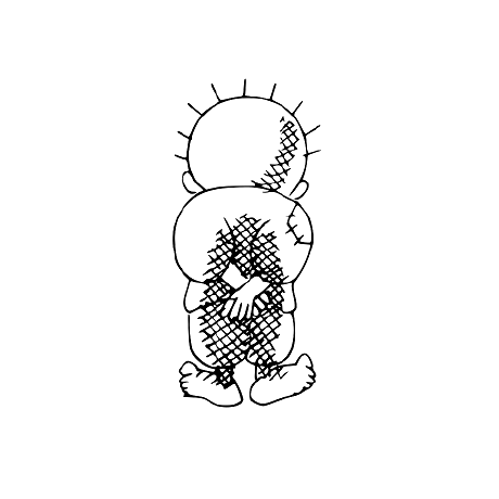
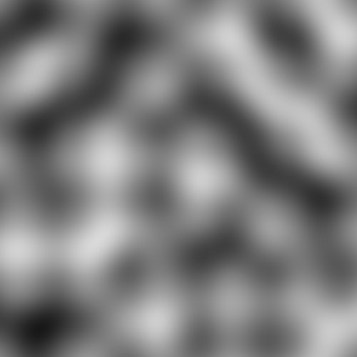
An interesting art project that Josh implemented:
the blue/red is perlin noise with quadratic interpolation, it looks like this up close:
Why we can’t use an LLM to generate the shader code?
I wouldn’t rely on a large language model (LLM) to generate shader code directly. Instead, I would opt for a structured approach using a library of routines designed to composite noise kernel outputs. These kernels could include Perlin, Worley, Simplex, or others. You could even start with a base texture and apply interpolation functions like linear, bilinear, spherical, sincos, or Lanczos. These functions provide a value between 0 and 1 at any fractional pixel position, and they can also work in 3D, which is especially useful for animated textures.
Once you have this value, you can map it to a color by passing it through a function that, for example, thresholds the output: values between 0 and 0.45 could correspond to blue, 0.45 to 0.55 to white, and 0.55 to 1 to red. However, these colors don’t have to be static; they can themselves be outputs from other noise functions, or simply raw textures or static colors, depending on the need. The final output can take various forms, such as a texture, U/V map, bump map, or normal map.
Essentially, this approach allows us to generate images with infinite detail by compositing noise kernels, textures, and colors. These generated images can then be used for various mapping purposes, like bump maps, normal maps, specular maps, or ambient textures. Tools like NeoTextureEdit already allow you to do much of this, though NeoTextureEdit is Java-based and generates only images, not shaders.
Once the procedural generation is fully developed, machine learning techniques could be applied to optimize the process, such as finding the best-fit procedural texture for a given target image. For example, if you wanted to generate something that resembles grass, you could use a genetic algorithm to find the noise kernel parameters that most closely approximate the texture of grass. The process could be initialized with several noise kernels selected via clustering methods like centroid or K-means. Applying K-means clustering over a tuple of DFT (Discrete Fourier Transform) values and color information could greatly improve the approximation of real-world textures. While these approaches involve machine learning, they don’t necessarily require deep neural networks (DNNs), but they would reduce the parameter space enough to make the application of DNNs feasible later on.
This Houdini page is interesting: https://www.sidefx.com/docs/houdini/nodes/sop/volumenoisesdf.html.
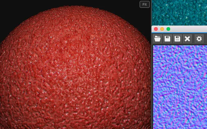
One of the great aspects of this project is that, by using shaders, you can instantly preview the same logic within a Qt GL context. This allows for rapid iterations and visual feedback.
Josh recommended incorporating the ability to modify the x, y, and z coordinates, as well as the final noise kernel value, using custom functions. For example, to create animations, you could introduce a time-based factor that shifts one or more of these values. This approach would enable dynamic changes and smooth transitions, making it easier to implement animated effects.
The most basic element is the ambient color map, or the primary texture that defines the surface appearance of an object. This map provides color information but doesn’t account for lighting or depth effects, so it can look flat, especially when viewed from different angles—similar to the visuals in games like Mario 64.
To enhance realism, additional techniques like specular mapping, offset mapping, and bump maps are applied. These techniques add depth, texture, and reflectivity to the surface, making it react more naturally to lighting and movement. See https://i.imgur.com/TgzU54D.jpeg.
By allowing users to define their texture as a normal map (or as a channel within a normal map), specular map, offset map, or even a bump map from which the others can be derived, we can unlock a range of visually impressive effects. This flexibility in handling texture mapping allows for more dynamic and realistic surfaces.
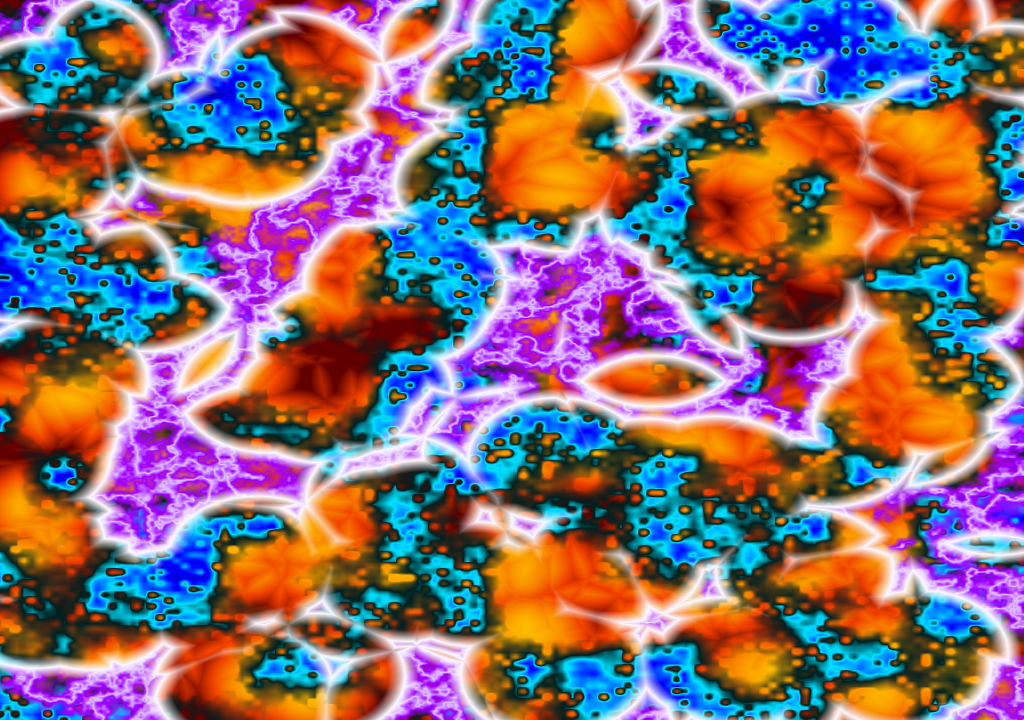
| Another interesting aspect is the use of Worley noise, which is distance-based. You can think of it as randomly-placed points, with each pixel representing the distance to the nearest point. One key variable is the distance function itself—it doesn’t have to be Cartesian (i.e., Euclidean distance, such as (\sqrt{(x_2 - x_1)^2 + (y_2 - y_1)^2})). You can use alternatives like Manhattan distance (( | x_2 - x_1 | + | y_2 - y_1 | )) or others, depending on the effect you want. Here’s a reference to various distance metrics: Numerics Mathdotnet Distance. |
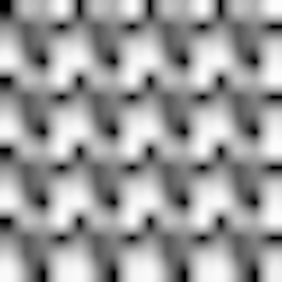
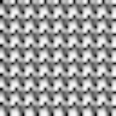
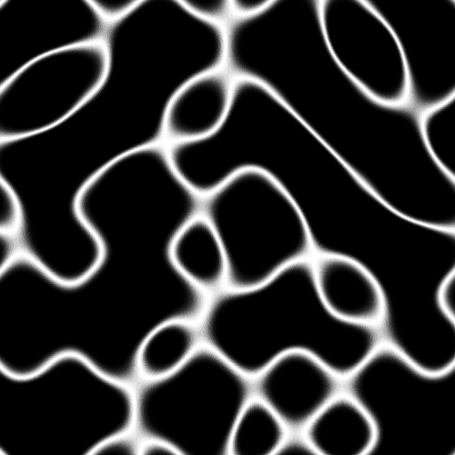
Another variable you can manipulate is the clamping function. The distance values you generate won’t naturally fall between 0 and 1; they could range up to the texture size. You can adjust how these values are clamped or even repeat the pattern. For instance, if you apply Worley noise with a Manhattan distance function and repeat every 20 units, you can achieve a pattern similar to the one in the image you referenced.
It’s worth noting that the example you shared probably has additional constraints, as some regions have distinct blackness around them. The exact distance function wasn’t shared, but the diagonal lines clearly indicate a Manhattan-based pattern. Chebyshev distance is another metric you might consider, though it wasn’t listed in the link.
Ultimately, my advice is to experiment—exploring how different mathematical operations on pixel data affect the visual outcome is not only educational but also a lot of fun. You can use this exploration to create stunning fractals, patterns, and shaders. Essentially, what I’m suggesting is a tool or wizard that sits on top of ShaderToy, providing users with an accessible interface for these kinds of shader manipulations.
Imagine a 4x4 random texture and scaling it up; something like this:

that’s just cubic interpolation
here’s linear:

and here’s none:

watch what happens if I tile it to 8×8, 16×16, 32×32, upscale all to 400×400:


when I composite those (via addition), I get this:
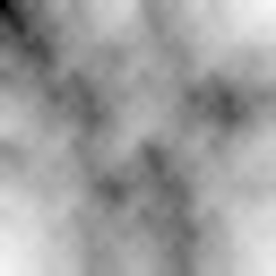
mind you, that’s very regular-looking because I made it entirely by hand there’s nothing random about it, really but you can see how I started with a 4x4 grid of “random” pixels, upsampled to 400×400 with a lanczos interpolation function (“LoHalo”), then composited so in that routine, the final output is .5 (octave 1) + .25 (octave 2) + .125 (octave 3) + .0625 (octave 4)
Josh used Gimp to create the images.
Seif — 22/02/2024 19:58
magnificent … u can create a cold mountain view using just the right noise function … I really loved that art this is my first time dealing with something that describes “perfection” as “not needed” else we need something random not perfect, this is so cool
Josh — 22/02/2024 20:34
now you’re getting it 🙂 our goal here is to put this power in users’ hands we want it to be easy for them to discover how useful this is perlin noise is used in things like enemy layout, too (edited) it controls resource deposits in games like Terraria and Factorio
For example:
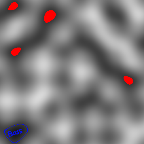
enemy camps where the red is, boss camp where the blue is, walls around it in blue just as an example
Josh showed me another example:
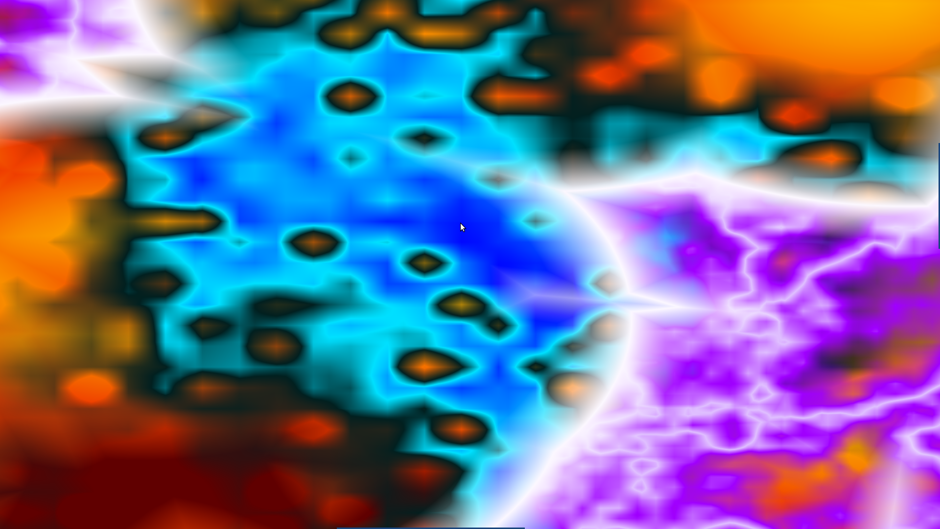
oh, and I think you’ve probably figured this out by now, but look what happens if you take that same image I pasted above and make only a small band in the middle white:
so a really cool way to animate this is by sliding that pass band around (changing the accepted/white values from 0-0.1 gradually up to 0.1-0.2 and continuing to 0.2-0.3 … 0.5-0.6 … 0.9-1) the other way to animate it is to use a 3D grid and move slowly along the Z axis (which you can do with or without that pass band)
This is a great example of reflections at the bottom of a pool or perhaps a visualization of an electrical field.
A great example of this project’s output would be: https://acegikmo.com/shaderforge/
The last technical issue I want to address is the problem of generating infinite textures using Worley noise. Josh suggested solving this by applying the modulo operator, which I’ve also detailed in my proposal.
Worley noise works by choosing random point locations in advance, but the challenge is that this inherently limits the texture to a finite area. My initial suggestion was to place these points in a random grid, but there’s a catch: not every grid cell should necessarily contain a point, and the point’s position within the cell should be randomized. The issue arises when you have only a limited number of points (N). Without tiling those points, you can’t generate pixels beyond their containing area, which prevents the texture from being infinite.
To overcome this limitation, we can use a pseudo-random function based on the coordinates (x, y) to determine whether a grid cell contains a point, and if so, where that point is positioned within the cell. While this method ensures infinite generation, it eliminates the possibility of multiple points being clustered together in close proximity, which is a trade-off.
“Tiling” refers to a technique where, for example, in a 128×128 texture, the point at (130,130) would correspond to the same point at (2,2) by using the modulus operation to wrap the coordinates. The challenge here is that points will appear constrained to their respective grid cells, which may produce a visually artificial pattern. However, this can be mitigated with more complex mathematical techniques.
One effective solution to improve tileability is to introduce multiple octaves of noise. By doing this, you progressively increase the freedom of point movement. For instance, 50% of the points could be restricted to their grid cell, 75% could move freely within the surrounding 8x8 cells, 87.5% within 64x64 cells, and so on. By the time you’re looking at a 512x512 region, 93.75% of the points are still bound, but the human eye would likely be unable to detect these constraints. This multi-octave approach creates a more natural and seamless texture across infinite space.